Model fitting for variable domain functional data • VDPO

Introduction

The VDPO package provides, among other tools, methods for analyzing variable domain functional data. This vignette demonstrates how to fit variable domain functional regression models using the vd_fit function, which is designed to handle various types of functional and non-functional covariates in a flexible framework.

Data Generation

library(VDPO)

We’ll start by generating sample data using the data_generator_vd function. This function creates simulated data with variable domain functional covariates and additional non-functional covariates if specified.

# Generate data with functional and non-functional covariates
data <- data_generator_vd(beta_index = 1, use_x = TRUE, use_f = TRUE)

Model Fitting

The vd_fit function is the main tool for fitting variable domain functional regression models. It supports various model specifications through a formula interface.

Basic Model with Single Functional Covariate

Let’s start with a basic model using only the functional covariate:

data <- data_generator_vd(beta_index = 1, use_x = FALSE, use_f = FALSE)
formula <- y ~ ffvd(X_se, nbasis = c(10, 10, 10))
res <- vd_fit(formula = formula, data = data)

Model with Multiple Functional Covariates

If your data contains multiple functional covariates, you can include them in the model:

data <- data_generator_vd(
  beta_index = 1,
  use_x = FALSE,
  use_f = FALSE,
  multivariate = TRUE
)
formula <- y ~ ffvd(X_se, nbasis = c(10, 10, 10)) + ffvd(Y_se, nbasis = c(10, 20, 10))
res_multi <- vd_fit(formula = formula, data = data)

Model with Functional and Non-Functional Covariates

The vd_fit function also supports including non-functional covariates, both linear and smooth terms:

data <- data_generator_vd(beta_index = 1, use_x = TRUE, use_f = TRUE)
formula <- y ~ ffvd(X_se, nbasis = c(10, 10, 10)) + f(x2, nseg = 30, pord = 2, degree = 3) + x1
res_complex <- vd_fit(formula = formula, data = data)

In this model:

ffvd(X_se, nbasis = c(10, 10, 10)) specifies the functional covariate
f(x2, nseg = 30, pord = 2, degree = 3) adds a smooth effect for x2
x1 is included as a linear term

Model Summary

You can obtain a summary of the fitted model using the summary function:

summary(res_complex)
#> 
#> Family: gaussian 
#> Link function: identity 
#> 
#> 
#> Formula:
#> NULL
#> 
#> 
#> Fixed terms: 
#>                                  x2                                     
#>   1.4678062   0.9742174  -0.1430355  -3.5265899   5.2136636 -10.5801911 
#>             
#>   6.0838833 
#> 
#> 
#> Estimated degrees of freedom:
#> Total edf     Total      <NA>      <NA>      <NA> 
#>    4.9380    4.5461    0.0001    9.4842   16.4842 
#> 
#> R-sq.(adj) =  0.958   Deviance explained = 97.5%  n = 100
#> 
#> Number of iterations: 1

Working with Non-Aligned Data

The vd_fit function can handle both aligned and non-aligned functional data. Here’s an example with non-aligned data:

data_not_aligned <- data_generator_vd(aligned = FALSE, beta_index = 1)
formula <- y ~ ffvd(X_se, nbasis = c(10, 10, 10))
res_not_aligned <- vd_fit(formula = formula, data = data_not_aligned)

Additional functionality

If you need to include an offset in your model, you can use the offset argument:

offset <- rnorm(nrow(data$X_se))
res_with_offset <- vd_fit(formula = formula, data = data, offset = offset)

Plotting the betas

A heatmap for a specific beta of the model can be obtained by using the plot function:

plot(res)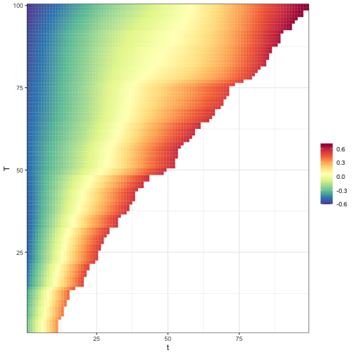

Final remarks

The vd_fit function in the VDPO package provides a flexible and powerful tool for fitting variable domain functional regression models. It supports a wide range of model specifications, including multiple functional covariates, non-functional covariates, and various distribution families. By leveraging the formula interface, users can easily specify complex models tailored to their specific analysis needs.